Processes
Processes provided by Rana
Every process in Rana is designed to streamline your workflow. Select your inputs, configure parameters, and let Rana handle the heavy lifting — whether you’re creating a DEM, generating boundary conditions, or launching a rainfall-runoff simulation.
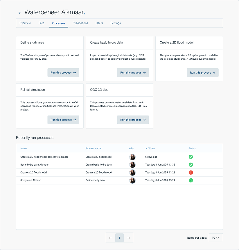
Rana has the following processes available:
Recently Ran processes
In recently ran processes you’ll find the processes ran in the project by any user in that project.
In Process Runner the input and output of the process is stated
In Status are the log messages during the running of the process
In Results is a preview of the result
Define Study Area
Create a valid study area polygon for your project. It extracts one or more polygons from a layer, merges them into one and (optionally) adds a buffer around it.
The resulting polygon can be used as “study area” input in other processes related to hydrological modelling, data analysis, or visualization.
For your convenience, Rana provides datasets of administrative boundaries that you can choose from. You may also use any other polygon layer from your project.
Create Basic Hydrodata
Add essential hydrological datasets to your project.
The process extracts elevation, soil, and land cover raster datasets for your study area and adds them to your project. These layers allow you to quickly conduct a hydrological scan of your study area.
Select your study area and the datasets you need, and the outputs will be automatically aligned to the correct spatial projection for seamless integration into your project.
The outputs are raster files that cover your whole study area.
Create 2D Flood Model
Create a flood model for your study area, ready for use in assessment of flooding due to intense rainfall (pluvial flooding). This Rana model is also a reliable foundation for further analyses: integrated urban drainage assessments, coastal and/or fluvial flooding studies, and more. Simply open it in the Rana Desktop Client to have the full range of expert modelling options at your fingertips.
The output of this process
The output is a 2D hydrodynamic model that allows you to simulate rainfall, infiltration, runoff, overland flow, ponding and flooding. This output becomes the basis for rainfall and flow analysis simulations in follow-up processes.
Technical documentation Study area requirements
Outputs of the process Define study area is guaranteed to be a valid input for this process. If you use another file as input, it has to meet these requirements:
It contains a single layer with a single polygon in it.
It has a projected coordinate reference system, with meters as unit.
The polygon is within the Netherlands.
Model The resulting Model is a 2D Model with a DEM and spatially variable friction coefficients and infiltration capacities. The DEM is taken at the highest available resolution. The computational cell size will be chosen in such a way that the model will have around 50,000 computational cells.
Optionally: A buffer of 50 meters will be added to the study area. DEM pixels in this buffer will be given a value of 50 m below the lowest value in the DEM to ensure that water can flow out of the study area, into this buffer. This ensures a realistic water flow in the study area and prevents artificial flooding at the edges of your study area.
Simulate Rainfall
This process allows you to simulate constant rainfall scenarios for one or Rana model in your project. The simulation starts with a rain period where a constant rain intensity is applied across the entire model. After the rain period ends, the simulation continues with a dry period, allowing you to observe water retention, runoff, and drainage behavior. This type of simulation is essential for analyzing how the terrain and landscape respond to sustained rainfall events, helping identify potential flooding risks and evaluating water management strategies.
Simulate rainfall event: standard events NL
Simulate Rainfall Event: Standard Events (Netherlands) This process allows you to simulate a standard rainfall event used in the Netherlands. These are C2100 rainfall events from RIONED for one Rana model in your project.
The input of this process
Model, a rana model, for example created by the ‘Create 2D flood model’ process.
Rainfall event, select a C2100 rainfall event.
Raw simulation results
These files can be used for advanced analysis in the Rana Desktop Client. These files contain the water levels, volumes, flow velocities, discharge, and other relevant variables for each output time step of the simulation (for example, every 5 minutes). For more information, see Rana Documentation.
Technical documentation
A schematisation may have multiple revisions; the Rana model of the latest revision is used in the simulation. A Rana model for the latest revision will be generated if it does not exist yet.
If multiple simulation templates exist for the Rana model, the most recent one will be used.
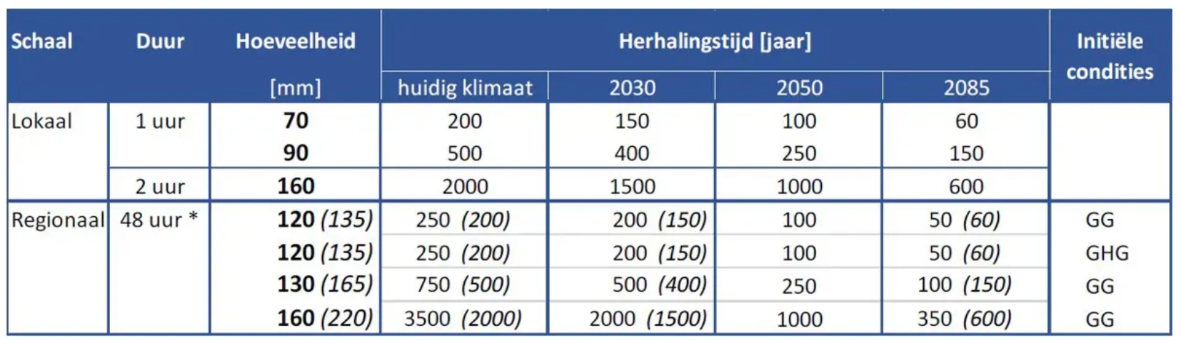
Overview standard rainfall events
Simulate rainfall events: constant
This process allows you to simulate a constant rainfall event, used as a stress test in the Netherlands. These events are determined by RIONED.
The input of this process
Model, a rana model, for example created by the ‘Create 2D flood model’ process.
Rainfall event, select a historical rainfall event.
Processed simulation results
Max water depth, in meters relative to the surface (DEM). The exact moment that this maximum water depth occurs can vary between cells.
A scenario result, that can be readily used in a publication.
Detailed NetCDF files, that can be used for further analysis in the Rana Desktop Client.
Raw simulation results
These files can be used for advanced analysis in the Rana Desktop Client. These files contain the water levels, volumes, flow velocities, discharge, and other relevant variables for each output time step of the simulation (for example, every 5 minutes). For more information, see Rana Documentation.
Technical documentation
A schematisation may have multiple revisions; the Rana model of the latest revision is used in the simulation. A Rana model for the latest revision will be generated if it does not exist yet.
If multiple simulation templates exist for the Rana model, the most recent one will be used.
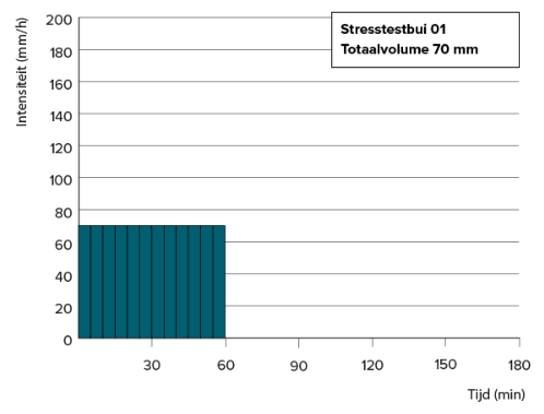
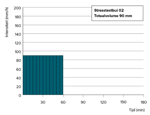
Overview constant rainfall events
The figures of the source of these events are visible below the figures.
DPRA event 70 mm
DPRA event 90 mm
90 mm
DPRA event 160 mm
160 mm
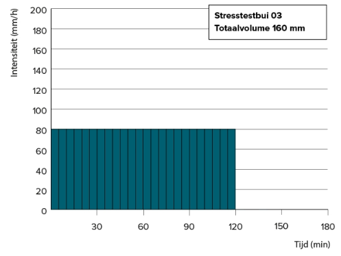
For more information about these rainfall events please visit the website of RIONED. Note that for that an account is needed, then the URL can be accessed here: https://www.riool.net/kennisbank/onderzoek/modelleren-hydraulisch-functioneren/stap-iv-hydraulische-belasting-bepalen/hemelwaterafvoer-hwa/ontwerpbuien-met-statistische-herhalingstijd/stresstestbuien
Simulate rainfall events: historical:
This process allows you to simulate a historic rainfall event for one schematization in your project.
The input of this process
Model, a rana model, for example created by the ‘Create 2D flood model’ process.
Rainfall event, select a historical rainfall event.
Processed simulation results
Max water depth, in meters relative to the surface (DEM). The exact moment that this maximum water depth occurs can vary between cells.
A scenario result, that can be readily used in a publication.
Detailed NetCDF files, that can be used for further analysis in the Rana Desktop Client.
Raw simulation results
These files can be used for advanced analysis in the Rana Desktop Client. These files contain the water levels, volumes, flow velocities, discharge, and other relevant variables for each output time step of the simulation (for example, every 5 minutes). For more information, see Rana Documentation.
Technical documentation
A schematisation may have multiple revisions; the Rana model of the latest revision is used in the simulation. A Rana model for the latest revision will be generated if it does not exist yet.
If multiple simulation templates exist for the Rana model, the most recent one will be used.
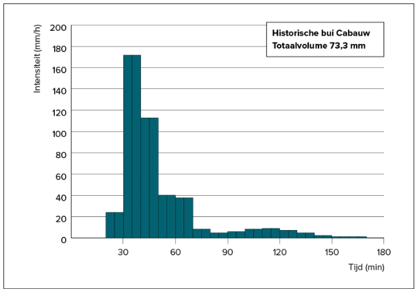
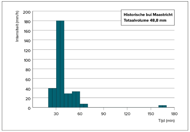
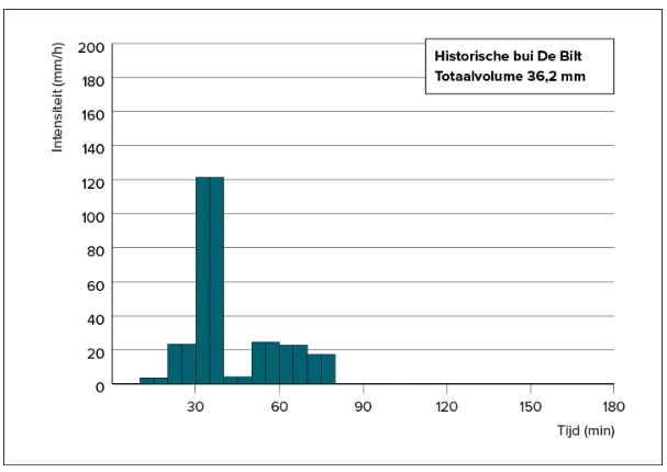
Overview historical rainfall events
Historical rainfall event name |
Total rainfall (mm) |
Rainfall event duration (h) |
Time series duration (h) |
Timestep (min) |
Year measurements |
Return period |
Source |
|---|---|---|---|---|---|---|---|
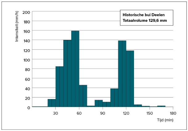
Deelen |
129.6 |
2 hours and 50 minutes |
2 hours and 50 minutes |
5 |
2014 |
T=1000 |
Rioned |
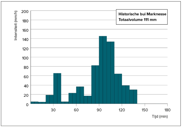
Marknesse |
111.0 |
2 hours and 20 minutes |
2 hours and 50 minutes |
5 |
2003 |
T=500 |
Rioned |
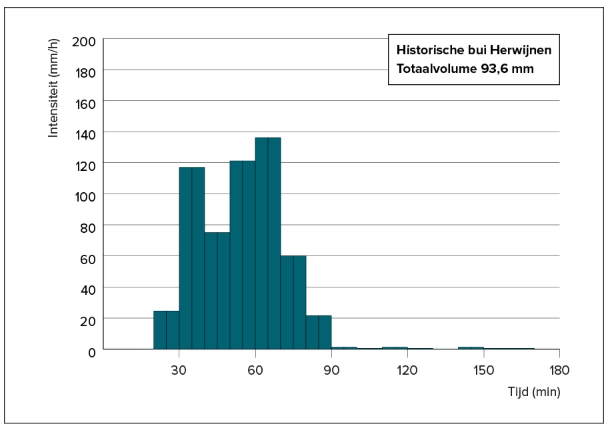
Herwijnen |
93.6 |
2 hours and 30 minutes |
2 hours and 50 minutes |
5 |
2011 |
T=500 |
Rioned |
Cabauw |
73.3 |
2 hours and 30 minutes |
2 hours and 50 minutes |
5 |
2005 |
T=200 |
Rioned |
Maastricht |
48.8 |
2 hours and 30 minutes |
2 hours and 50 minutes |
5 |
2014 |
T=100 |
Rioned |
De Bilt |
36.2 |
1 hour and 10 minutes |
2 hours and 50 minutes |
5 |
2016 |
T=20 |
Rioned |
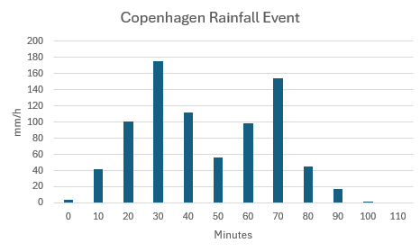
Copenhagen |
134.5 |
1 hour and 50 minutes |
1 hour and 50 minutes |
10 |
2011 |
T>2000 |
DMI / Arnbjerg-Nielsen et al. |
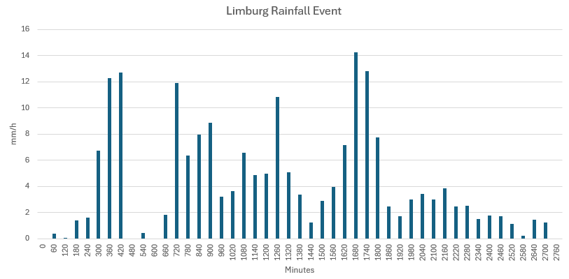
Limburg |
200.4 |
48 hours |
49 hours |
60 |
2021 |
T=1000 |
Stowa |
Details Historical Event Deelen
Details Historical Event Marknesse
Details Historical Event Herwijnen
Details Historical Event Cabauw
Details Historical Event Maastricht
Details Historical Event De Bilt
Details Historical Event Copenhagen
Details Historical Event Limburg
In July 2021, Limburg experienced an extreme rainfall event that led to significant flooding, primarily caused by a storm depression named ‘Bernd.’ This unprecedented rainfall resulted in the Meuse and Geul rivers overflowing, damaging thousands of homes and infrastructure, and causing estimated losses of 350 to 600 million euros. The event was characterized by record-breaking precipitation levels, making it one of the most severe flooding incidents in the region’s history.
More information about the first six rainfall events please visit the web page of RIONED. Note that for that an account is needed, then the URL can be accessed here: https://www.riool.net/kennisbank/onderzoek/modelleren-hydraulisch-functioneren/stap-iv-hydraulische-belasting-bepalen/hemelwaterafvoer-hwa/gemeten-neerslag/historisch-gemeten-buien-voor-stresstest.
The source of the last event is from the Danish Institute of Meteorology, and was accessed using their API using the following URL: https://opendataapi.dmi.dk/v2/metObs/collections/observation/items?stationId=05735¶meterId=precip_past10min&datetime=2011-07-02T17:10:00Z/2011-07-02T18:50:00Z&limit=11 (16-1-2026).
The source of the Limburg event can be found here https://klimaatadaptatienederland.nl/hulpmiddelen/overzicht/handreiking-bovenregionale-stresstesten/ when clicking the PDF (17-03-2026).
Assess Building flood risk
This process analyzes flood risk for individual buildings by combining simulation results with building footprint data. It calculates which buildings are vulnerable to flooding and provides detailed risk assessments based on simulated water levels and building characteristics.
Example result:
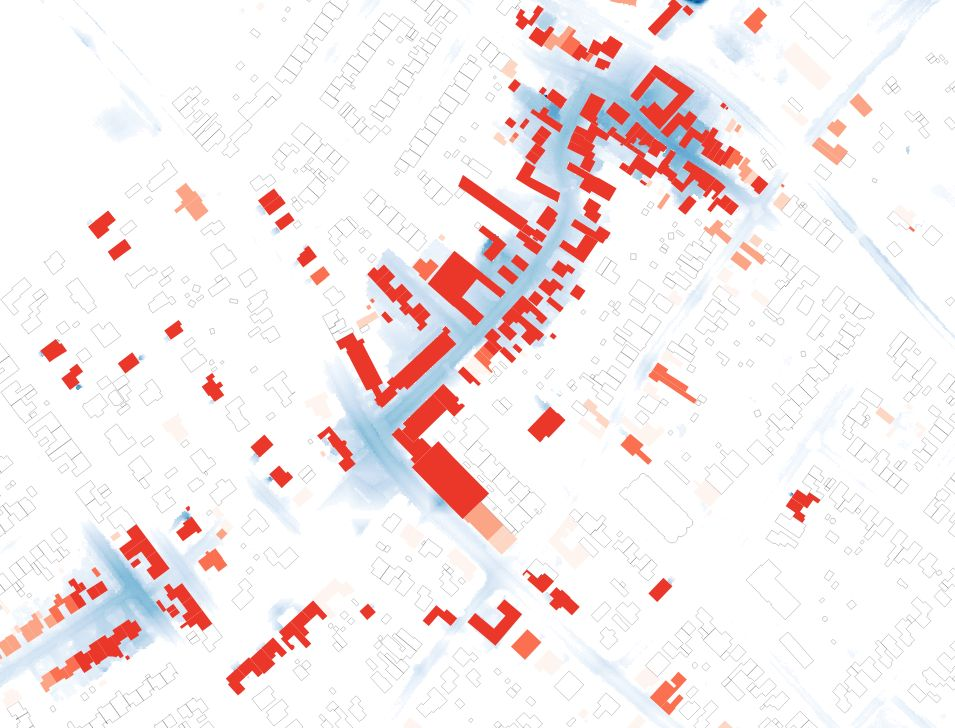
The process takes simulation results (scenario data) and building vector data as inputs, then determines flood impact for each building.
Scenario
A scenario file containing simulated water level data from previous flood simulation processes. This provides the time series water levels needed to assess flood impact on buildings.
Buildings Vector File
A vector file containing building footprints with the following requirements:
Supported formats: Shapefile, GeoJSON, or other OGR-compatible formats
Must contain single polygon geometries representing individual buildings
Must have a defined coordinate reference system (CRS)
Must contain only a single layer
Calculation Method
Basic Method (DGBC): Provides general flood risk assessment without considering building floor levels. Every building is buffered with 2 meters. Based on water depths around the buildings, buildings are classified as follows:
Water depth around the building |
Classification |
Description |
|---|---|---|
0m |
Class 0 |
No Flood Risk |
0-0.1 m |
Class 1 |
Very Low Risk |
0.1-0.15 m |
Class 2 |
Low Risk |
0.15-0.2 m |
Class 3 |
Moderate Risk |
0.2-0.3 m |
Class 4 |
High Risk |
The output of this process
Flood Risk Results
A vector file (.gpkg) containing the original building footprints enhanced with flood risk analysis results. Each building polygon includes calculated flood risk metrics based on the simulation data and selected calculation method.
Technical Documentation
Building Vector Requirements
The buildings vector file must meet specific criteria:
Single layer containing building footprint polygons
Defined coordinate reference system with appropriate projection
Single polygon geometries only (no multi-polygons or other geometry types)
Flood Risk Calculation
The process analyzes simulation results against building locations to determine:
Which buildings are affected by flooding
Flood depth at building locations
Risk assessment based on water levels and building characteristics
The calculation considers the temporal aspects of flooding from the scenario data to provide comprehensive flood impact analysis for each building in the dataset
Extract dataset
Import a dataset (for instance a digital elevation model) into your project. Select your study area and the dataset you need, and the output will be automatically aligned to the correct spatial projection for seamless integration into your project.
Compute water depth difference
This process calculates the difference in water depth between two raster files representing water depth data. It takes a reference water depth raster and a comparison raster as inputs, computes the difference (comparison minus reference) for their overlapping area, and outputs a new raster file with the result.
This process is useful for analyzing changes in water depth over time or between different scenarios, helping you identify areas where water levels have increased or decreased.
The input of this process
Water depth reference raster: The baseline water depth raster for comparison.
Water depth raster to compare The water depth raster to compare against the reference.
The output of this process
Water depth difference raster: A raster showing the calculated difference in water depth between the two input rasters. Positive values indicate areas where water depth increased, while negative values indicate areas where water depth decreased.
Technical documentation
Requirements
Both input rasters must have the same pixel size and coordinate reference system
Rasters should have overlapping geographic areas for meaningful comparison
Calculation Method
The process computes the difference as: comparison raster - reference raster
Data Handling
Areas with no data are treated as zero water depth
If rasters have different extents, only the overlapping area is processed
Create 3D water level data
Convert simulation results to a water level layer in a format that can be used in 3D platforms (OGC 3D Tiles).
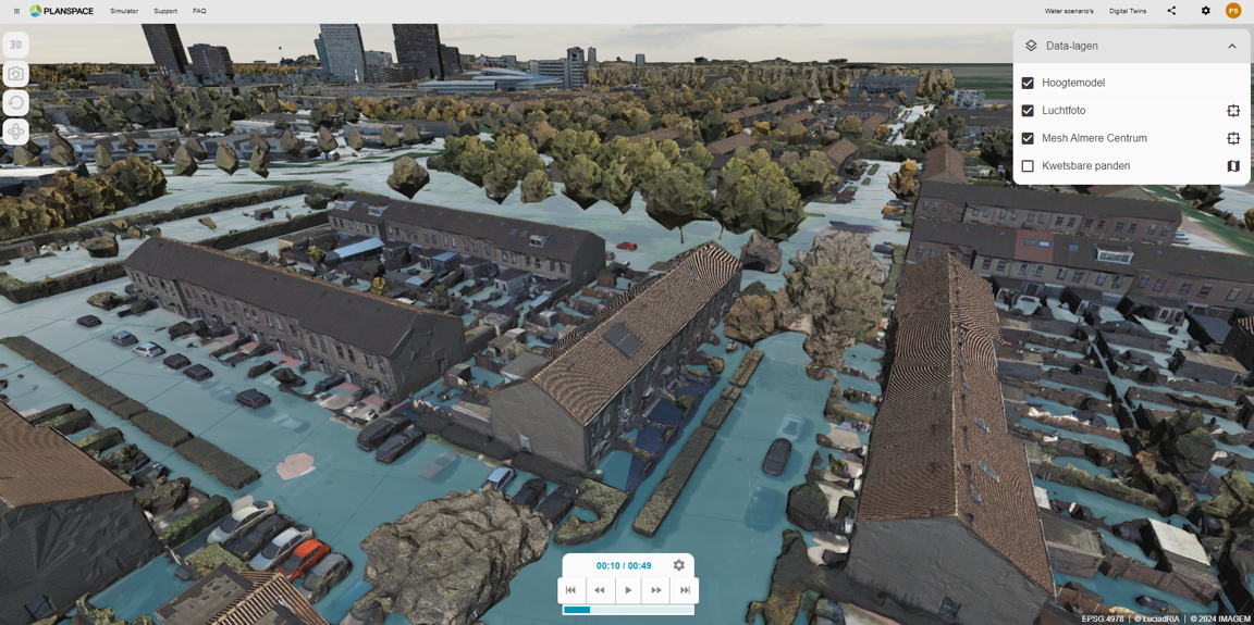
Note
The image above shows 3D visualisation in 3rd party software. Rana only provides the OGC 3D Tiles, other software is required to be able to visualise them.
Visualizing water levels in 3D can help stakeholders make better decisions regarding flood risks, infrastructure planning, and water management strategies. OGC 3D tiles make this possible. The format efficiently handles large datasets, allowing users to view and interact with 3D models without performance issues.
The output of this process
An OGC 3D Tiles file with water level surfaces. This file can be viewed in GIS platforms or web viewers to visualize the simulation results.
The input of this process
Interval (in seconds) between tile frames: This input defines the time gap between each frame (or snapshot) of water levels in the 3D tiles. A shorter interval resuts in smoother animations but generates more data and larger files.
Select a Scenario: A simulation result from which the water level data will be read. Use for example the Rainfall simulation process to create this file.
Calculate drainage pattern
Extract the main overland drainage routes from a digital elevation model. The drainage pattern gives immediate, visual insight in the hydrological behaviour of your study area. Each streamline also contains a list of attributes such as the Strahler order and the distance to outlet, that can be used for further analysis.
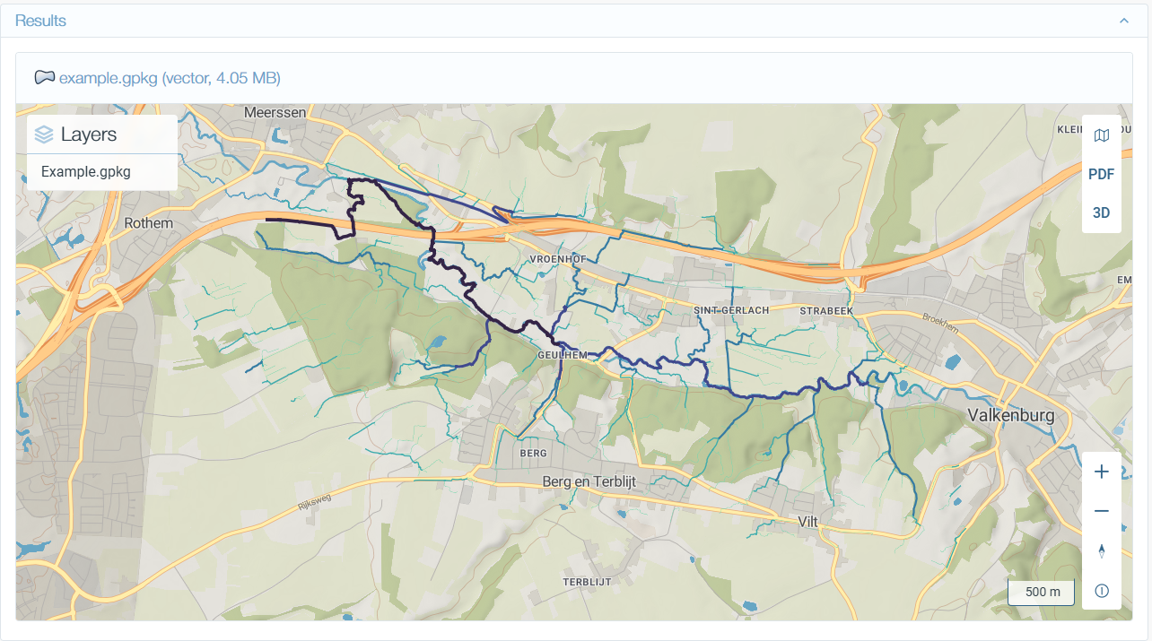
A minimum catchment area [m²] can be specified. A smaller number will result in more streamlines being returned by the algorithm. With a larger number, only the streamlines draining a larger area will be returned.
The output of this process
The output is a vector layer of streamlines. For an explanation of its attributes, see the Whitebox documentation.
Technical documentation
This analysis tool chains a number of algorithms from Whitebox Geospatial:
Breach depressions least cost
Fill depressions
D8 pointer
D8 flow accumulation
Extract streams
Raster streams to vector
Vector stream network analysis
The result is copied to a geopackage layer with easier to understand field names. Gaussian smoothing is applied to the lines. The smoothing does not affect the first and last vertex of each line, i.e. topology is preserved.
Delineate basins
Delineate basins (watersheds) from a digital elevation model. Basins are defined as areas that drain to the same edge pixel. The basins can be used to help you understand the hydrological functioning of your study area, or to subdivide a large area in smaller, hydrologically separate study areas.
The output of this process
The output is a vector layer of basin polygons.
Technical documentation
This analysis tool chains a number of algorithms from Whitebox Geospatial:
Breach depressions least cost
Fill depressions
D8 pointer
Basins
The result is vectorized and copied to a geopackage layer “basins”. Gaussian smoothing is applied to the polygons. The smoothing preserves topology (creates no gaps or overlaps).
Rana process damo2hydamo
Converts water management data from the DAMO format to the HyDAMO standard used in the Netherlands. It takes a DAMO file (containing information about water systems like canals, pumps, and water levels) along with two configuration files that define the data structures, and transforms everything into a clean, standardized HyDAMO file. During the conversion, it translates cryptic codes into readable descriptions, adds proper identification numbers to all water objects, and ensures the data meets current Dutch water management standards - making it easier to share data between different organizations and software tools.
Calculate floor levels
Calculate floor levels This process calculates floor levels of individual buildings, given the digital elevation map (DEM). It does so by sampling the DEM 1 meter around the building and taking the 75 percentile of the elevation values.
The output is a geopackage with 1 layer that has the ‘floor_level’ column added.
Prepare Digital Elevation From AHN
Extract and process Dutch elevation data (AHN - Actueel Hoogtebestand Nederland) to prepare a digital elevation model with calculated floor levels for buildings in your study area.
This process downloads the specified AHN dataset, fills missing elevation values, calculates floor levels around building footprints, and produces a final elevation raster suitable for hydrological modeling.
The output of this process
A GeoTIFF raster file containing the digital elevation model with integrated floor level data for buildings, clipped to your study area boundaries. The floor level represents the estimated ground surface elevation around each building, which is essential for accurate flood risk assessment and water flow modeling.
The input of this process
Study Area A polygon vector dataset defining the geographic extent for elevation data extraction. This ensures all processed data corresponds to your specified area of interest.
Buildings Vector File A vector file containing building footprints with polygon geometries representing individual buildings. Supported formats include Shapefile, GeoJSON, or other OGR-compatible formats. If your file contains multiple layers, you can specify which layer contains the building footprints.
AHN Version and Data Type Version: Select from AHN versions 2-6 Data Type: Choose between DTM (Digital Terrain Model - terrain only) or DSM (Digital Surface Model - includes surface features like vegetation and structures) Resolution The cell size (in meters) for the output raster. The default resolution depends on the selected AHN version. You can also specify a custom cell size to balance accuracy and file size.
Floor Level Calculation Parameters
Distance: The buffer distance (in meters) around each building footprint used to sample elevation values
Percentile: The statistical percentile (0-100) used to determine floor level. For example, 75 means the floor level is set such that 75% of the buffered area is below this elevation
Decimal Precision: The number of decimal places for rounding interpolated elevation values
Technical documentation
The process performs several sequential steps:
Data Validation: Validates that the study area polygon and buildings vector file are properly formatted
AHN Extraction: Downloads and extracts the specified AHN dataset clipped to study area boundaries
Data Interpolation: Fills missing or null elevation values using interpolation techniques to create a continuous DEM
Floor Level Calculation: For each building, buffers the footprint, samples elevation values within the buffer, and computes the percentile-based floor level
Rasterization: Converts calculated floor level values back onto the DEM raster
Final Processing: Clips the result to study area boundaries and optimizes file size
The elevation raster uses a metric coordinate reference system, which is validated during processing. All interpolated values are rounded to the specified decimal precision for consistent data.
Generate D-Hydro Freeboard
Calculates corrected freeboard (drooglegging) values. Combining model outputs with storage node effects, and filters out boezem (lake/buffer water) areas.
The input of this process
- Boezem (Lake / Buffer Water)Shapefile / GeoPackage
Boezem (lake/buffer water) polygons to exclude from analysis.
Source: D-Hydro model input or water management area definitions.
Required: Polygon geometry representing water bodies.
- Calculation Points (WITH storage nodes)GeoPackage
Calculation points with water levels from D-Hydro model (WITH storage nodes).
Source: D-Hydro FlowFM output (_his.nc files).
Required columns: ‘t_end’ (water level), geometry (point locations).
- Water Levels WITHOUT Storage NodesCSV
Water levels without storage node effects.
Source: D-Hydro FlowFM output (separate run without storage nodes).
Format: Skip first row (metadata), column ‘Water level - mesh1d_nNodes: mean (m)’.
- Freeboard CSV (WITHOUT storage)CSV
Model freeboard values at calculation points (calculated WITHOUT storage nodes).
Source: D-Hydro FlowFM output (run without storage nodes).
Formula: Good freeboard = freeboard_without_storage + (wl_without_storage - wl_with_storage)
Format: Skip first row (metadata), column ‘Freeboard - mesh1d_nNodes: mean (m)’.
The output of this process GeoPackage with corrected freeboard values:
Layer ‘freeboard_winter’: Corrected freeboard (fb_cor = freeboard + waterstand).
Layer ‘freeboard_zomer’: Empty layer (placeholder for future summer calculations).
Points in boezem areas set to -9999 (nodata).
Compute Max Water Depth
This process calculates the maximum water depth raster from a Rana HCC scenario file. It takes a scenario archive as input, extracts the required simulation files, computes the maximum water depth over time, and outputs a raster file with the result.
This process is useful for identifying the highest flood depths reached during a simulation, helping you assess flood impact and support risk analysis.
The input of this process
HCC Scenario file: A Rana scenario archive containing simulation results.
The output of this process
Max water depth raster: A raster showing per pixel the maximum water depth reached during the simulation. Higher values indicate deeper inundation.
Technical documentation
Requirements
The scenario archive must contain a GridAdmin file (.h5)
The scenario archive must contain a results file (.nc)
The scenario archive must contain a DEM file (.tif)
Calculation Method
The process computes maximum water depth using HCC depth calculation on the scenario input files.
Data Handling
The scenario archive is downloaded and extracted before processing
The result is written as a GeoTIFF raster (max_waterdepth.tif)